library(ggplot2)

# Paramètre
p <- 0.3

# Support
x <- c(0, 1)
p_x <- dbinom(x, size = 1, prob = p)
F_x <- pbinom(x, size = 1, prob = p)Lois de probabilité discrètes
Lois usuelles
1 Loi de Bernoulli
Loi de Bernoulli de paramètre (p) :
\[ X \sim \mathcal{B}(p) \]
Support : \(X \in {0,1}\)
Espérance : \[\mathbb{E}[X]=p\]
Variance : \[\mathbb{V}[X]=p(1-p)\]
Fonction de masse : \(\mathbb{P}(X=x)=p^x(1-p)^{1-x},\quad x\in{0,1}\)
Code
ggplot(data.frame(x = factor(x), prob = p_x), aes(x = x, y = prob)) +
geom_col(fill = "darkcyan", width = 0.02) +
scale_y_continuous(name = "P(X = x)", limits = c(0,1)) +
labs(title = "Fonction de masse de la loi de Bernoulli (p = 0.3)",
     x = "x")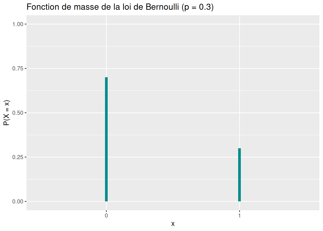
Code
ggplot(data.frame(x = x, cdf = F_x), aes(x = x, y = cdf)) +
geom_step(color = "darkcyan", linewidth = 1.5) +
scale_x_continuous(breaks = x) +
scale_y_continuous(name = "F(x)", limits = c(0,1)) +
labs(title = "Fonction de répartition de la loi de Bernoulli (p = 0.3)",
     x = "x")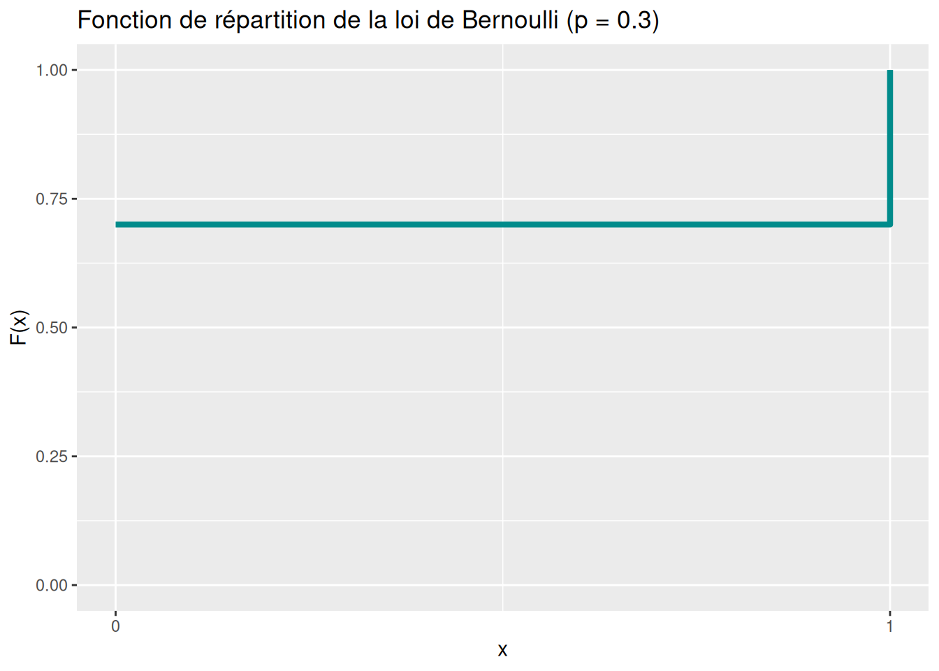
Générer un échantillon de n réalisations suivant la loi \(\mathcal{B}(p)\)
n <- 5
ech <- rbinom(n, size = 1, prob = p)
data.frame(ech)
import numpy as np
import pandas as pd
ech = np.random.binomial(n=1, p=0.3, size=5)
pd.DataFrame(ech, columns=["echantillon"])Fonction génératrice des probabilités :
\[G_X(s)=\mathbb{E}[s^X]=(1-p)+ps\]
Fonction caractéristique :
\[\phi(t)=(1-p)+pe^{it}\]
Propriétés :
- Somme de Bernoulli i.i.d. :\(\sum_{i=1}^n X_i \sim \mathcal{B}(n,p)\)
- Cas limite : \(X \sim \mathcal{B}(p)\Rightarrow 1-X \sim \mathcal{B}(1-p)\)
2 Loi Binomiale
Loi binomiale de paramètres \(\n\in\mathbb{N}^\*\) et \(p\in[0,1]\) : \(X \sim \mathcal{B}(n,p)\)
Interprétation : nombre de succès dans n épreuves de Bernoulli indépendantes de paramètre p.
Espérance : \[\mathbb{E}[X]=np\]
Variance : \[\mathbb{V}[X]=np(1-p)\]
library(ggplot2)

# Paramètres
n <- 10
p <- 0.3

# Support
x <- 0:n
p_x <- dbinom(x, size = n, prob = p)
F_x <- pbinom(x, size = n, prob = p)
Fonction de masse : \(\mathbb{P}(X=k)=\binom{n}{k} p^k (1-p)^{n-k},\quad k=0,\dots,n\)
Code
ggplot(data.frame(x = x, prob = p_x), aes(x = x, y = prob)) +
geom_col(fill = "darkcyan", width = 0.1) +
scale_x_continuous(breaks = x) +
scale_y_continuous(name = "P(X = k)") +
labs(title = "Fonction de masse de la loi Binomiale (n = 10, p = 0.3)",
     x = "k")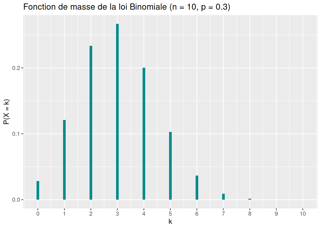
Code
ggplot(data.frame(x = x, cdf = F_x), aes(x = x, y = cdf)) +
geom_step(color = "darkcyan", linewidth = 1.5) +
scale_x_continuous(breaks = x) +
scale_y_continuous(name = "F(k)") +
labs(title = "Fonction de répartition de la loi Binomiale (n = 10, p = 0.3)",
     x = "k")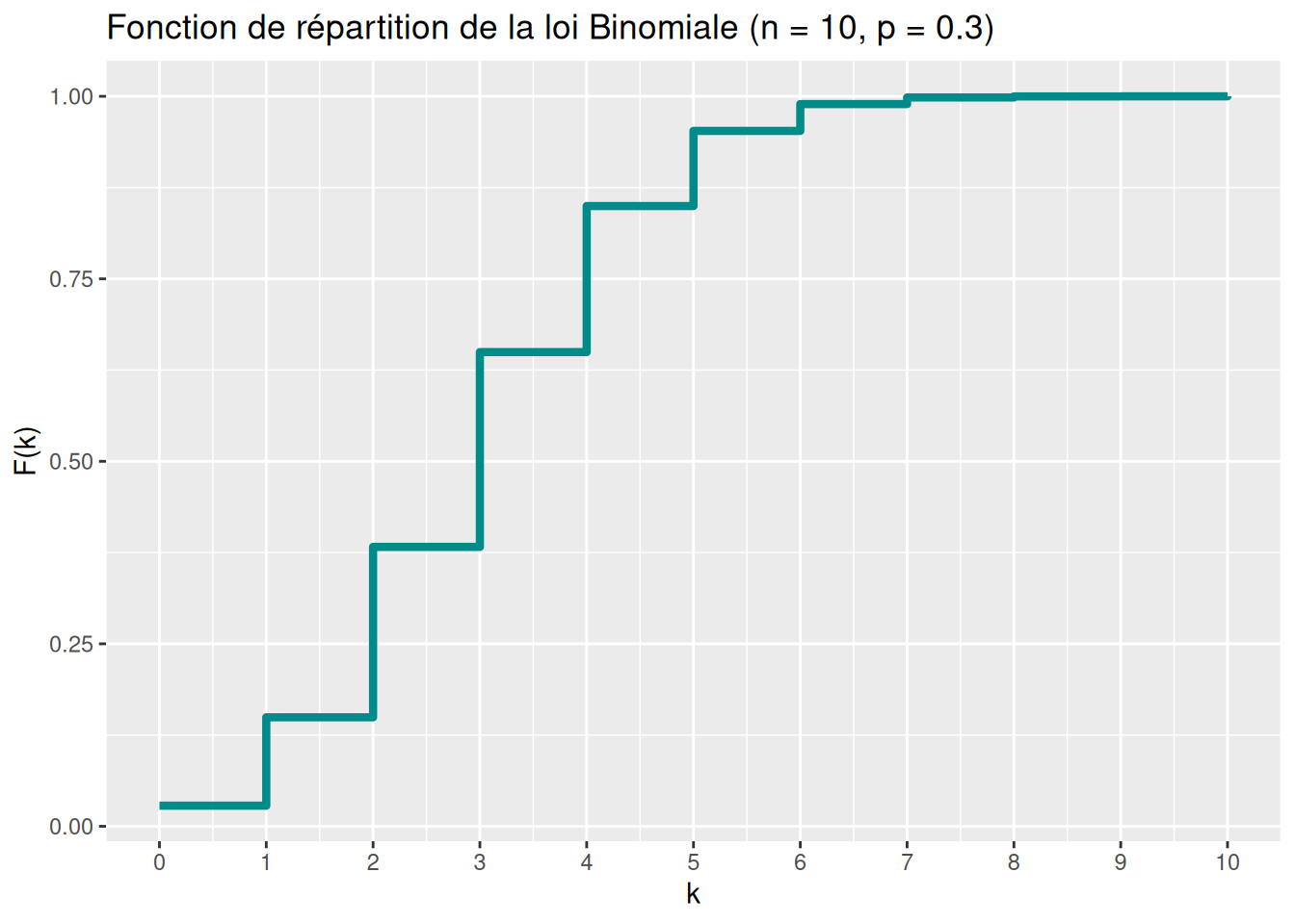
Générer un échantillon de m réalisations suivant la loi \(\mathcal{B}(n,p)\)
m <- 5
ech <- rbinom(m, size = n, prob = p)
data.frame(ech)
import numpy as np
import pandas as pd
ech = np.random.binomial(n=10, p=0.3, size=5)
pd.DataFrame(ech, columns=["echantillon"])Fonction génératrice des probabilités : \(G_X(s)=\mathbb{E}[s^X]=(1-p+ps)^n\)
Fonction caractéristique : \(\phi(t)=(1-p+pe^{it})^n\)
Propriétés :
- Somme de Bernoulli : \(\sum_{i=1}^{n} X_i \sim \mathcal{B}(n,p)\) avec \((X_i)\) i.i.d. Bernoulli
- Approximation de Poisson : \(\mathcal{B}(n,p)\approx \mathcal{P}(np)\) si n grand et p petit
- Approximation normale : \(\mathcal{B}(n,p)\approx \mathcal{N}(np,np(1-p))\) si \(np(1-p)\) grand
3 Loi de Poisson
Loi de Poisson de paramètre \(\lambda>0\) : \[X \sim \mathcal{P}(\lambda)\] Espérance : \[\mathbb{E}[X]=\lambda\] Variance : \[\mathbb{V}[X]=\lambda\]
library(ggplot2)

# Paramètre

lambda <- 3

# Support

x <- 0:15
p_x <- dpois(x, lambda = lambda)
F_x <- ppois(x, lambda = lambda)
Fonction de masse : \[\mathbb{P}(X=k)=\frac{\lambda^k}{k!}e^{-\lambda},\quad k\in\mathbb{N}\]
Code
ggplot(data.frame(x = x, prob = p_x), aes(x = x, y = prob)) +
geom_col(fill = "darkcyan", width = 0.1) +
scale_x_continuous(breaks = x) +
scale_y_continuous(name = "P(X = k)") +
labs(title = "Fonction de masse de la loi de Poisson (λ = 3)",
     x = "k")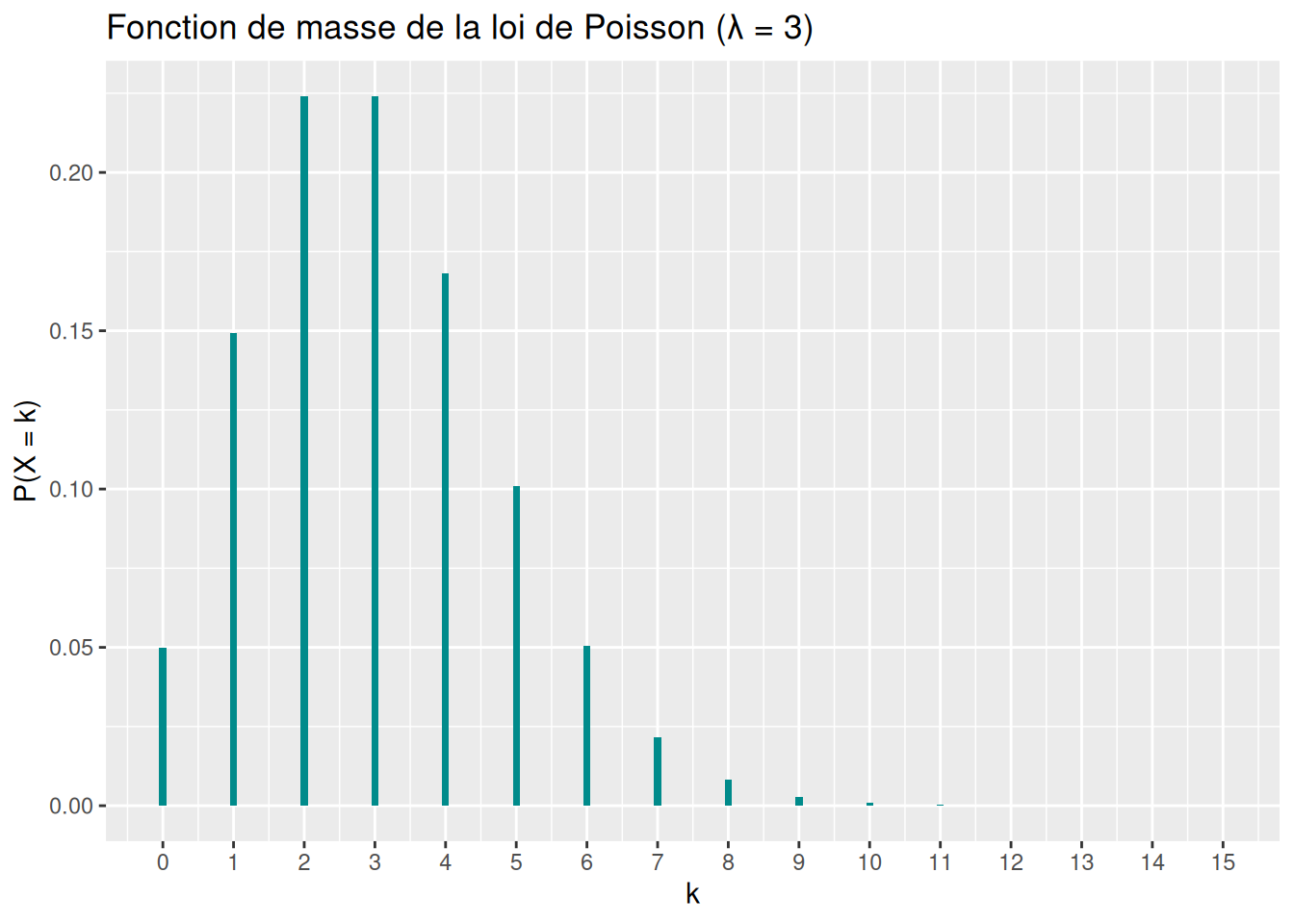
Code
ggplot(data.frame(x = x, cdf = F_x), aes(x = x, y = cdf)) +
geom_step(color = "darkcyan", linewidth = 1.5) +
scale_x_continuous(breaks = x) +
scale_y_continuous(name = "F(k)") +
labs(title = "Fonction de répartition de la loi de Poisson (λ = 3)",
     x = "k")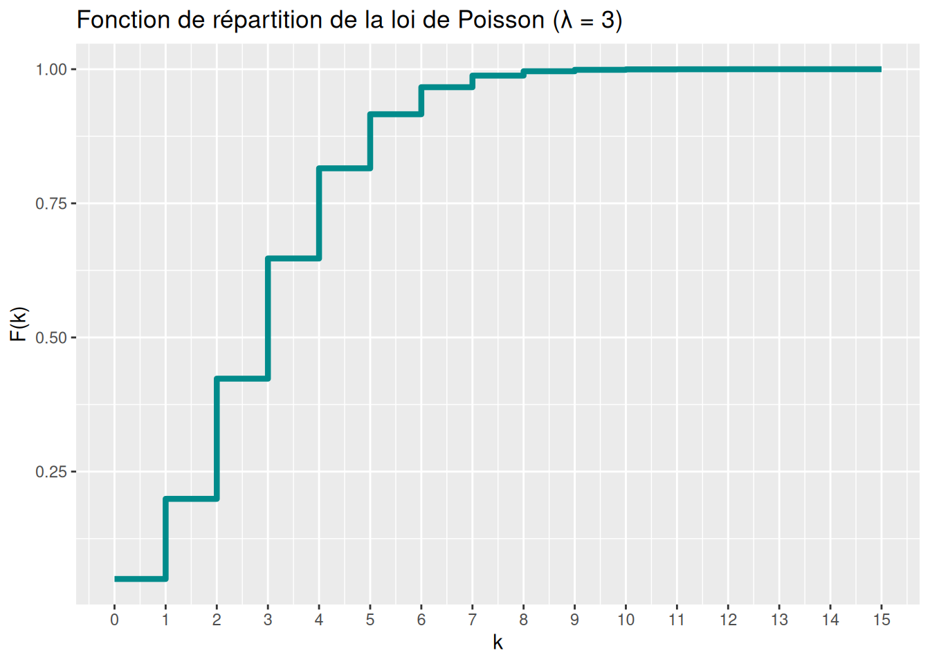
Générer un échantillon de n valeurs suivant la loi \(\mathcal{P}(\lambda)\)
n <- 5
ech <- rpois(n, lambda = lambda)
data.frame(ech)
import numpy as np
import pandas as pd
ech = np.random.poisson(lam=3, size=5)
pd.DataFrame(ech, columns=["echantillon"])Fonction génératrice des probabilités : \[G_X(s)=\mathbb{E}[s^X]= \exp\big(\lambda(s-1)\big)\]
Fonction caractéristique : \[\phi(t)=\exp\big(\lambda(e^{it}-1)\big)\]
Propriétés :
- Additivité : Si $X_1(_1) et \(X_2\sim\mathcal{P}(\lambda_2)\) et $\(X_1\perp X_2\) \(\Rightarrow X_1+X_2\sim\mathcal{P}(\lambda_1+\lambda_2)\)
- Approximation :\(\mathcal{B}(n,p)\approx\mathcal{P}(np) \quad \text{si } n\text{ grand et }p\text{ petit}\)