library(ggplot2)

# Paramètres
mu <- 0
sigma2 <- 1

# Générer des points à tracer
x <- seq(mu - 3, mu + 3, length.out = 100)
f_x <- dnorm(x, mean = mu, sd = sigma2)
F_x <- pnorm(x, mean = mu, sd = sigma2)Lois de probabilité continues
Lois usuelles
1 Loi Normale
Loi Normale de moyenne \(\mu\) et de variance \(\sigma^2\) :
\[\mathcal {N}(\mu,\sigma^2)\]
Densité : \[f(t)=\frac{1}{\sqrt{2 \pi \sigma^2}} e^{-\frac{1}{2} \frac{(t-\mu )^{2}}{\sigma ^{2}}}\]
Code
# Tracer la courbe avec ggplot2
ggplot(data.frame(x = x, density = f_x), aes(x = x, y = density)) +
  geom_line(color = "darkcyan", linewidth = 1.5) +
  scale_x_continuous(name = "x", limits = c(-3, 3)) +
  scale_y_continuous(name = "f(x)") +
  labs(title = "Densité de la loi Normale(0, 1)")
Code
# Tracer la courbe avec ggplot2
ggplot(data.frame(x = x, cdf = F_x), aes(x = x, y = cdf)) +
  geom_line(color = "darkcyan", linewidth = 1.5) +
  scale_x_continuous(name = "x", limits = c(-3, 3)) +
  scale_y_continuous(name = "F(x)") +
  labs(title = "Fonction de répartition de la loi Normale(0, 1)")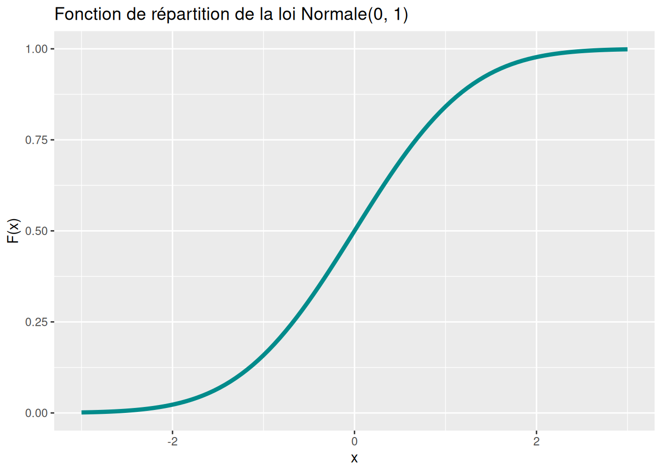
Générer un échantillon de n valeurs suivant la loi \(\mathcal{N}(0,1)\)
n <- 5
ech <- rnorm(n, mean = 0, sd = 1)
data.frame(ech)
Warning
Le dernier paramètre est l’écart-type, pas la variance !
import numpy as np
import pandas as pd

ech = np.random.normal(loc=0, scale=1, size=5)

pd.DataFrame(ech, columns=["echantillon"])
Warning
Le dernier paramètre est l’écart-type, pas la variance !
Fonction caractéristique : \[\phi (t)={\rm {e}}^{\mu {\rm {i}}t-{\frac {1}{2}}\sigma ^{2}t^{2}}\]
Propriétés : \[X_1 + X_2 \sim \mathcal{N}(\mu_1 + \mu_2,\sigma_1^2 + \sigma_2^2) \Leftrightarrow {\begin{cases}X_1 \sim \mathcal{N}(\mu_1,\sigma_1^2) \\ X_2 \sim \mathcal{N}(\mu_2,\sigma_2^2) \\ X \perp \!\!\! \perp Y \end{cases}}\]
2 Loi Uniforme Continue
Loi uniforme continue sur l’intervalle ([a,b]) :
\[\mathcal{U}(a,b)\]
Espérance : \[\mathbb{E}[X]=\frac{a+b}{2}\]
Variance : \[\mathbb{V}[X]=\frac{(b-a)^2}{12}\]
library(ggplot2)

# Paramètres
a <- 0
b <- 1

# Générer des points à tracer
x <- seq(a - 0.2, b + 0.2, length.out = 200)
f_x <- dunif(x, min = a, max = b)
F_x <- punif(x, min = a, max = b)
Densité : \[f(x)=\frac{1}{b-a} \mathbb{1}_{a \leq x \leq b}(x)\]
Code
ggplot(data.frame(x = x, density = f_x), aes(x = x, y = density)) +
geom_line(color = "darkcyan", linewidth = 1.5) +
scale_x_continuous(name = "x") +
scale_y_continuous(name = "f(x)") +
labs(title = "Densité de la loi Uniforme(0,1)")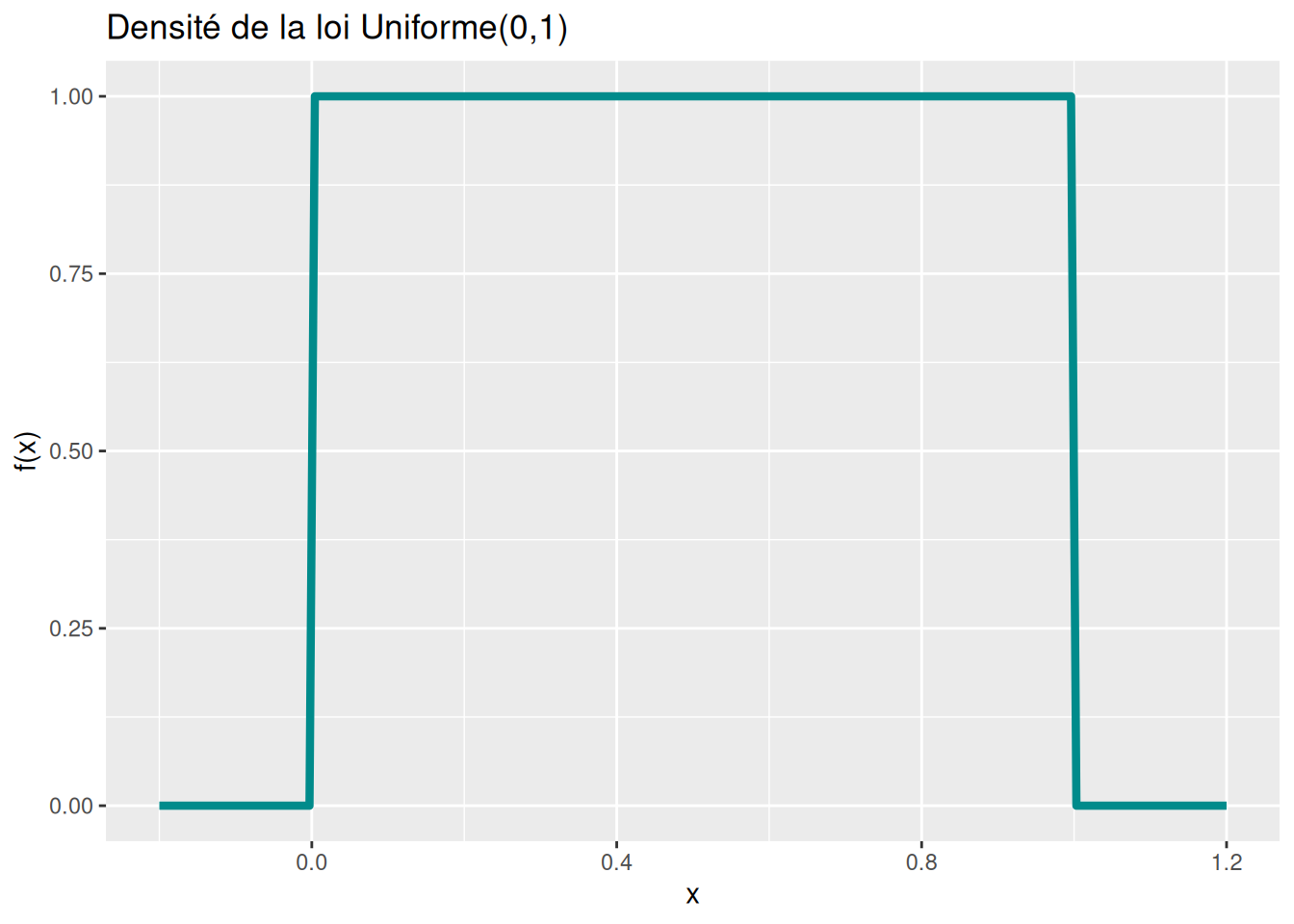
\[F(x)={\begin{cases}0&{\text{pour }}x<a\\{\dfrac {x-a}{b-a}}&{\text{pour }}a\leq x<b\\1&{\text{pour }}x\geq b\end{cases}}\]
Code
ggplot(data.frame(x = x, cdf = F_x), aes(x = x, y = cdf)) +
geom_line(color = "darkcyan", linewidth = 1.5) +
scale_x_continuous(name = "x") +
scale_y_continuous(name = "F(x)") +
labs(title = "Fonction de répartition de la loi Uniforme(0,1)")
Générer un échantillon de n valeurs suivant la loi \(\mathcal{U}(a,b)\)
n <- 5
ech <- runif(n, min = a, max = b)
data.frame(ech)
import numpy as np
import pandas as pd
ech = np.random.uniform(low=0, high=1, size=5)
pd.DataFrame(ech, columns=["echantillon"])Fonction caractéristique : \[\phi(t) = \frac {{\rm {e}}^{{\rm {i}}tb}-{\rm {e}}^{{\rm {i}}ta}}{{\rm {i}}t(b-a)}\]
Propriétés :
- Si \(X\sim\mathcal{U}(a,b)\), alors \(\frac{X-a}{b-a}\sim\mathcal{U}(0,1)\)
- Transformation affine : \(\alpha X+\beta \sim \mathcal{U}(\alpha a+\beta,\alpha b+\beta) \quad (\alpha>0)\)
3 Loi du \(\chi^2\)
Loi du \(\chi^2\) à \(k\) degrés de liberté :
\[\chi^2(k) \sim \sum_{i=1}^{k} X_i^2 \quad \text{avec } X_i \sim \mathcal{N}(0,1)\ \text{i.i.d.}\]
Espérance : \[\mathbb{E}[\chi^2(k)] = k\]
Variance : \[\mathbb{V}[\chi^2(k)] = 2k\]
library(ggplot2)

# Paramètre
k <- 3

# Générer des points à tracer
x <- seq(0, 20, length.out = 300)
f_x <- dchisq(x, df = k)
F_x <- pchisq(x, df = k)
Densité : \[f(t)=\frac{1}{2^{k/2}\Gamma(k/2)}t^{k/2-1} e^{-t/2}\mathbb{1}_{t \ge 0}\]
Code
# Paramètres
df_values <- c(1, 2, 3, 5, 10, 20)

# Genérer des données
data <- lapply(df_values, function(df) {
  x <- seq(0, 30, length.out = 200)
  f_x <- dchisq(x, df = df)
  data.frame(x = x, density = f_x, df = as.factor(df))
})
data <- do.call(rbind, data)

# Tracer la courbe avec ggplot2
ggplot(data, aes(x = x, y = density, color = df)) +
  geom_line(linewidth = 1) +
  scale_x_continuous(name = "x", limits = c(0, 30)) +
  scale_y_continuous(name = "f(x)") +
  labs(title = "Densité de la loi du Chi2 selon différents degrés de liberté") +
  scale_color_discrete(name = "df")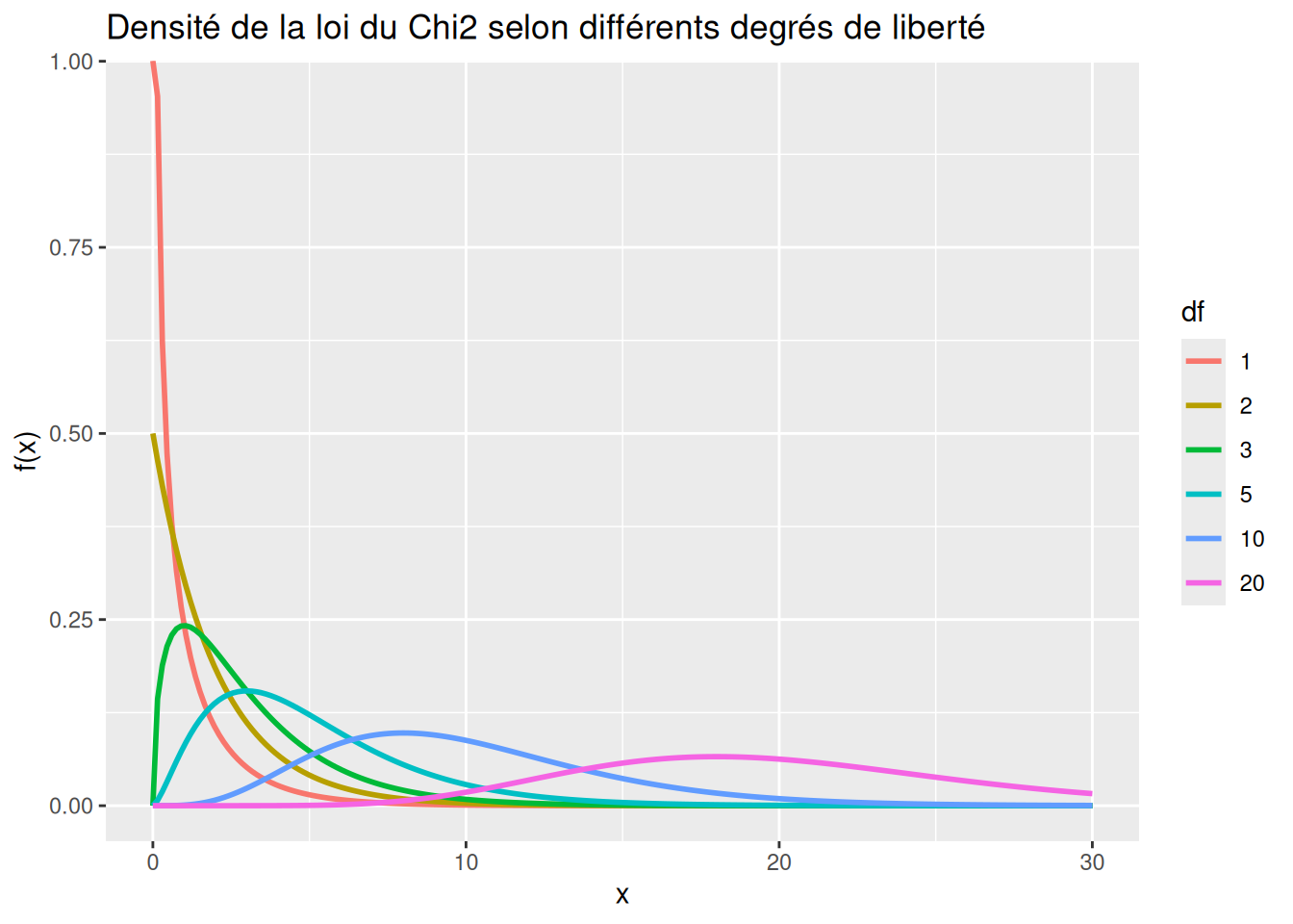
Code
ggplot(data.frame(x = x, cdf = F_x), aes(x = x, y = cdf)) +
geom_line(color = "darkcyan", linewidth = 1.5) +
scale_x_continuous(name = "x", limits = c(0, 20)) +
scale_y_continuous(name = "F(x)") +
labs(title = "Fonction de répartition de la loi du Chi² (k = 3)")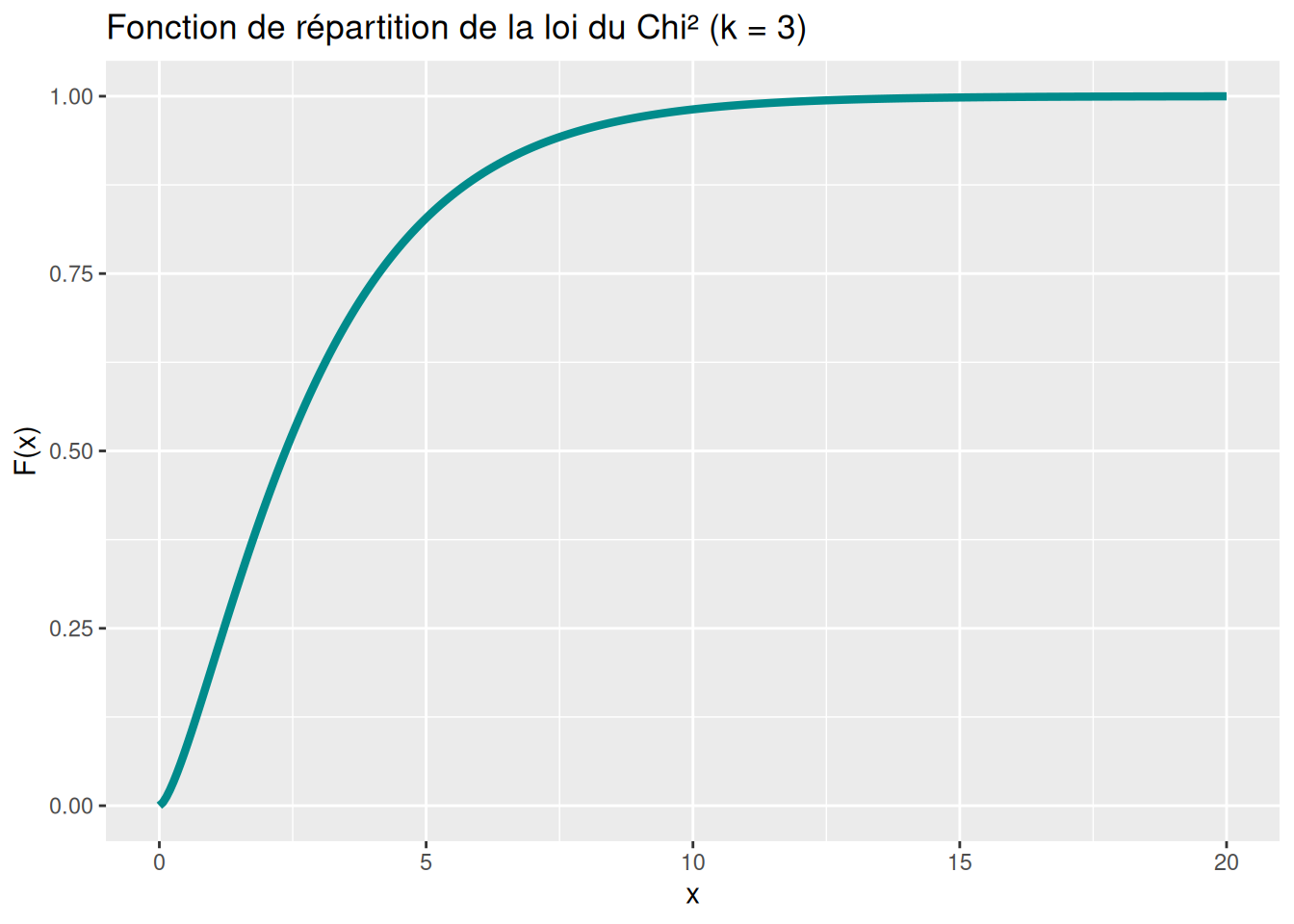
Générer un échantillon de n valeurs suivant la loi \(\chi^2(k)\)
n <- 5
ech <- rchisq(n, df = k)
data.frame(ech)
import numpy as np
import pandas as pd
ech = np.random.chisquare(df=3, size=5)
pd.DataFrame(ech, columns=["echantillon"])Fonction caractéristique : \[\phi(t) = (1-2it)^{-k/2}\]
Propriétés :
- Additivité : \(X_1 \sim \chi^2(k_1),\ X_2 \sim \chi^2(k_2),\ X_1 \perp X_2 ;\Rightarrow; X_1 + X_2 \sim \chi^2(k_1+k_2)\)
- Cas particulier : \(Z \sim \mathcal{N}(0,1) ;\Rightarrow; Z^2 \sim \chi^2(1)\)
4 Loi de Student
Loi de Student à n degrés de liberté.
\[\mathcal{T}(n) \sim \frac{\mathcal{N}(0,1)}{\sqrt{\chi^2(n)/n}}\]
Espérance : \[\mathbb{E}(\mathcal{T}(n)) = 0 \ si \ n > 1\]
Variance : \[\mathbb{V}(\mathcal{T}(n)) = \frac{n}{n-2} \ si \ n > 2 \ (+\infty \ sinon)\]
La loi de Student converge en loi vers la loi Normale \[\mathcal{T}(n) \underset{n \to +\infty}{\overset{\mathcal{L}} \longrightarrow} \mathcal{N}(0,1)\]
Code R
Code
library(ggplot2)

# Paramètres
df_values <- c(1, 2, 5, 20)

# Générer des données
data <- lapply(df_values, function(df) {
  x <- seq(-5, 5, length.out = 200)
  f_x <- dt(x, df = df)
  data.frame(x = x, density = f_x, df = as.factor(df))
})
data <- do.call(rbind, data)

# Tracer la courbe avec ggplot2
ggplot(data, aes(x = x, y = density, color = df)) +
  geom_line(linewidth = 1) +
  scale_x_continuous(name = "x", limits = c(-5, 5)) +
  scale_y_continuous(name = "f(x)") +
  labs(title = "Densité de la loi de Student selon différents degrés de liberté") +
  scale_color_discrete(name = "df")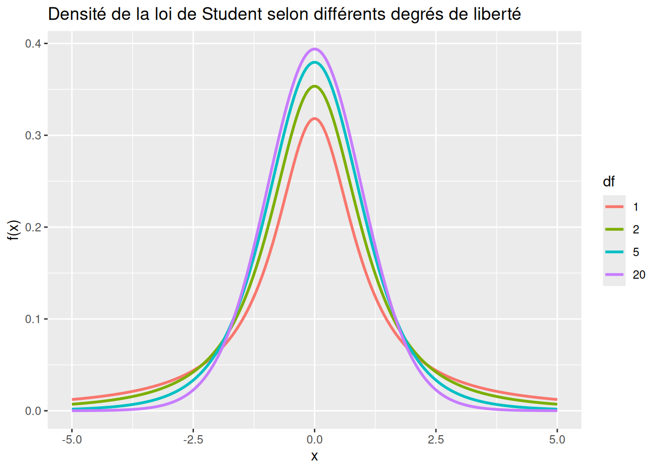
Générer un échantillon de n valeurs suivant la loi \(\mathcal{T}(df)\)
n <- 5
df <- 3
ech <- rt(n, df)
data.frame(ech)
5 Loi de Fisher-Snedecor
Loi de Fisher-Snedecor à n et m degrés de liberté
\(\mathcal{F}(n,m) \sim \frac{\chi^2(n)/n}{\chi^2(m)/m}\)
\(\mathbb{E}(\mathcal{F}(n,m)) = \frac {m}{m-2}\) si \(m > 2\)
\(X \sim \mathcal{F}(a,b) \Rightarrow \frac{1}{X} \sim \mathcal{F}(b,a)\)
Lien avec la loi de Student : \(X\sim \mathcal{T}(n) \Rightarrow X^2 \sim \mathcal{F}(1,n)\)
Lien avec la loi Normale : \(X \sim \mathcal{N}(0,1) \Rightarrow X^2 \sim \mathcal{F}(1,\infty)\)
6 Loi Exponentielle
Loi exponentielle de paramètre Lambda
\(\mathbb{E}(\epsilon(\lambda)) = \frac{1}{\lambda}\)
\(\mathbb{V}(\epsilon(\lambda)) = \frac{1}{\lambda^2}\)
Densité : \(\lambda e^{{-\lambda x}} \mathbb{1}_{x \geq 0}\)
Fonction de répartition : \(1-e^{{-\lambda x}}\)
Fonction caractéristique : \(\left(1-{\dfrac {it}{\lambda }}\right)^{{-1}}\)
7 Loi Gamma
Loi Gamma de paramètres alpha et beta
\(X \sim \Gamma( \alpha , \beta)\)
\(\mathbb{E}(\Gamma( \alpha , \beta)) = \frac{\alpha}{\beta}\)
\(\mathbb{V}(\Gamma( \alpha , \beta)) = \frac{\alpha}{\beta^2}\)
Densité : \(f ( x , \alpha, \beta ) = x^{\alpha -1} \frac{\beta ^\alpha e^{-\beta x}}{\Gamma (\alpha )} \mathbb{1}_{x > 0}\)
Liens avec d’autres lois :
- Si \(\alpha = 1 \sim\) loi exponentielle
- Si \(\Gamma (n / 2 , 1/2 ) \sim\) loi du \(\chi^2\) à \(n\) degrés de liberté
7.1 Fonction Gamma
\(\Gamma(a) = \int _{0}^{+\infty }t^{a-1}\,\mathrm {e} ^{-t}\,\mathrm dt\)
Prolonge la fonction factorielle à l’ensemble des nombres complexes (sauf entiers négatifs)
\(\Gamma(n+1) = n!\)
\(\Gamma(x+1) = x\Gamma(x)\)
7.2 Loi inverse Gamma
Loi inverse Gamma de paramètres k et \(\theta\)
\(X \sim {{Inv \ \Gamma}(k,\theta )} \Rightarrow \frac{1}{X} \sim \Gamma ( k , 1 / \theta )\)
Densité : \(f(x;\alpha ,\beta )={\frac {\beta ^{\alpha }}{\Gamma (\alpha )}}(1/x)^{\alpha +1}\exp \left(-\beta /x\right)\) pour \(x > 0\)
\(\mathbb{E}(Inv \ \Gamma( \alpha , \beta)) = \frac{\beta}{\alpha-1}\) pour \(\alpha > 1\)
\(\mathbb{V}(Inv \ \Gamma( \alpha , \beta)) = \frac {\beta ^{2}}{(\alpha -1)^{2}(\alpha -2)}\) pour \(\alpha > 2\)
8 Loi Beta
Loi Beta de paramètres alpha et beta
\(\mathbb{E}(\mathrm{B}) = \frac {\alpha }{\alpha +\beta }\)
\(\mathbb{V}(\mathrm{B}) = \frac {\alpha \beta }{(\alpha +\beta )^{2}(\alpha +\beta +1)}\)
Densité : \(\frac{x^{\alpha-1}(1-x)^{\beta-1}}{\mathrm{B} (\alpha ,\beta )}\)
8.1 Fonction Beta
\(\mathrm {B} (x,y)=\int _{0}^{1}t^{x-1}(1-t)^{y-1}\mathrm {d} t\)
\(\mathrm {B} (x,y)={\frac {\Gamma (x)\,\Gamma (y)}{\Gamma (x+y)}}\)
\(\mathrm {B} (x,y)=\mathrm {B} (y,x)\)
\(\mathrm {B} (x,y+1)=\frac{y}{x+y}\mathrm {B} (x,y)\)